Analysing Geological Data with Python and VRGS

Introduction: In the field of geology, analysing and visualising geological data is crucial for understanding various geological phenomena. In this blog post, we will explore how to utilise the embedded Python interpreter in VRGS to analyse and visualise geological data. We will walk through a Python code example that demonstrates the process of classifying geological attributes and creating a scatter plot to visualise the classified data.

To get started we need to load a VRGS project. Make sure you have a mesh dataset and have created some attributes. If you don't have Python 3.11 installed then install that on your machine. The installer is found here:

Download Python | Python.org

Go to the project properties (select the button from the top of the properties panel) and set the path to the python311 folder.

Getting Started: To begin, we need to install the VRGS library, which provides functionalities for accessing the data in VRGS. Once installed, we can import the necessary libraries in Python. In this case, we will use numpy and matplotlib, so you will need to pip-install those. The vrgs library is embedded in VRGS so there is no need to pip-install that one.

import vrgs
import matplotlib.pyplot as plt
import matplotlib as mpl
import numpy as np

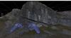
Data Classification: The first step in our analysis is to classify the geological attributes based on certain criteria. In the provided code, the classify function is defined to classify attributes dip and coplanarity. In this example, the criteria for classification are if the dip is greater than 60 (ie a steeply dipping surface) and coplanarity is greater than 4 (relatively planar). The function returns 1 for attributes that meet the criteria (a steeply dipping planar surface) and 0 otherwise. Please note this is a very simple and not particularly useful classification - you should update this function with your own method.

def classify(dip, coplanarity):
    if dip > 60 and coplanarity > 4:
        return 1
    else:
        return 0

The VRGS library functions for accessing point cloud and mesh data are outlined below:

# retrieve the list of meshes in the project - returns a list 
# of tuples with mesh name and its unique ID number
mesh_list = vrgs.mesh_list()


# return the list of x,y,z vertices for a mesh
mesh_vertices = mesh_vertices("mesh name")

# retrieve the list of attributes for a mesh
mesh_attribute_list = vrgs.mesh_attribute_list(mesh_list[0][0])

# return the list of values in the meshes attribute. Argument 1 is the 
# mesh nam and arument 2 is the attribute name. 
attribute = vrgs.mesh_attribute(mesh_list[0][0], mesh_attribute_list[0])

# more examples of retrieving attribute values
dip = vrgs.mesh_attribute(mesh_list[0][0], "Dip")
azimuth = vrgs.mesh_attribute(mesh_list[0][0], "Azimuth")
coplanarity = vrgs.mesh_attribute("Trefor Rocks", "CoPlanarity")

# To add a new attribute the arguments are mesh_name, name_of_new_attribute 
# and list_of_values.
vrgs.mesh_add_attribute("Trefor Rocks", "classified", result)

# equivalent commands for point clouds

pointcloud_vertices = vrgs.pointcloud_vertices("pointcloud name")
pcl_list = vrgs.pointcloud_list()
pcl_attribute_list = vrgs.pointcloud_attribute_list(pcl_list[0][0])
pcl_attribute = vrgs.pointcloud_vertices(pcl_list[0][0],pcl_attribute[0])
vrgs.pointcloud_attribute("pointcloud name", "new attribute name", result)

This library will be extended over time.

Data Retrieval and Analysis: The code then proceeds to retrieve the necessary geological data using the VRGS library. It fetches the list of meshes, mesh attributes, and specific attribute values for further analysis. The map function is used to apply the classify function to pairs of dip and coplanarity attributes, generating a list of classified results.

mesh_list = vrgs.mesh_list()
# ... Code to retrieve mesh attributes and specific attribute values ...

result = list(map(classify, dip, coplanarity))

Data Visualisation: Once the data is classified, we can create a scatter plot to visualise the results. The code uses the matplotlib library to create a scatter plot with coloured markers, where the size of the markers represents the classified result, ie the steeply dipping, high coplanarity values are plotted as larger points. To do this we multiply the classification result (0 or 1) by 50, then add 1, that way the sizes will be 1 and 51, rather than 0 or 50, so the unclassified points are actually plotted. We choose the inferno colour map in this case.

fig, ax = plt.subplots()
size = np.asarray(result)  * 50 + 1
cmap = mpl.cm.inferno
ax.scatter(dip, azimuth, c=coplanarity, s=size, cmap=cmap, alpha=0.05)
ax.set_xlabel('Dip', fontsize=15)
ax.set_ylabel('Azimuth', fontsize=15)
ax.set_title('Classified')
ax.grid(True)
fig.tight_layout()
plt.show()

When we run the final code in the VRGS Python window we get the following result:

The full code snippet is shown at the end of this page if you want to try it out yourself.

In this blog post, we explored how to utilise Python and the VRGS library to analyse and visualise geological data in the integrated Python editor. The provided code shows the process of classifying geological attributes based on dip and coplanarity, and creating a scatter plot to visualise the results. This workflow can be adapted and extended to analyse and visualise various geological datasets, providing valuable insights for geological studies and research.

Remember to install the necessary libraries and adapt the code to your specific geological dataset.

Happy exploring and analysing geological data with Python and VRGS!

import vrgs
import matplotlib.pyplot as plt
import matplotlib as mpl
import numpy as np

def classify(dip, coplanarity):
    if dip > 60 and coplanarity > 4:
        return 1
    else:
        return 0

mesh_list = vrgs.mesh_list()
if mesh_list:
    print(mesh_list)
    mesh_attribute_list = vrgs.mesh_attribute_list(mesh_list[0][0])
    if mesh_attribute_list:
        print(mesh_attribute_list)
        attribute = vrgs.mesh_attribute(mesh_list[0][0], mesh_attribute_list[0])
        if attribute:
            print(attribute[:20])
        dip = vrgs.mesh_attribute(mesh_list[0][0], "Dip")
        azimuth = vrgs.mesh_attribute(mesh_list[0][0], "Azimuth")
        coplanarity = vrgs.mesh_attribute("Trefor Rocks", "CoPlanarity")
        result = list(map(classify, dip, coplanarity))
        if result:
            print(result[:20])
            print(result.count(0))
            print(result.count(1))
        vrgs.mesh_add_attribute("Trefor Rocks", "classified", result)

        fig, ax = plt.subplots()
        size = np.asarray(result) * 50 + 1
        cmap = mpl.cm.inferno
        ax.scatter(dip, azimuth, c=coplanarity, s=size, cmap=cmap, alpha=0.05)
        ax.set_xlabel('Dip', fontsize=15)
        ax.set_ylabel('Azimuth', fontsize=15)
        ax.set_title('Classified')
        ax.grid(True)
        fig.tight_layout()
        plt.show()